
Understanding A/B Testing
A/B testing is a central tool of web analytics. Being able to incrementally improve your website is key to staying competitive online. What is so fascinating about A/B testing is that the fundamental concepts are easy to understand, yet mastering A/B-testing is very difficult.
In essence, A/B testing is a methodology to determine which variant of two is more effective. It has become a wildly popular tool in web analytics for improving websites. It usually involves modifying an element of a website (such as a headline or image) to see if the alteration ups the website’s performance. For an e-commerce website, improving its conversion rate could lead to ever so important increased sales.
With the introduction of accessible experiment design softwares, such as Google Optimize, almost anyone can have an A/B-test up and running in no time. Although this is generally good, the task of setting up A/B-tests has become so streamlined and automated that tests are conducted even when they should not, mainly due to insufficient data (could be both in terms of quantity and quality).
To become good at A/B-testing one must learn how to conduct reliable tests, when to (not) conduct tests, and how to interpret the results. Especially when it comes to the first two activities, the test tools do little to help. This is why some deeper knowledge of the statistics behind A/B-testing often is necessary.
As I have experienced, getting started with statistics can be very overwhelming, especially to learn the seemingly endless terminology. But don’t worry, I’m here to help you get started. This will be the first part of (at least) two, where I will explain the process and some fundamental statistical concepts of A/B testing. The ambition of this blog series is not to provide a complete guide of everything related to A/B testing, but rather to educate those unfamiliar on the subject. In the first part of the series I focus on the methodology and core concepts that make up an A/B test, while the second part will cover different types of statistical tests and how they should be used. Let’s get started!
Overview
There will be lots of ground to cover when it comes to the concept and structure of A/B testing. So in this blog I have focused on the components that I believe are the most fundamental for getting started. I will not go into too much detail about any of the concepts instead I have focused on the pure basics. In case you would like to learn more about some of the concepts additional links are provided. I have divided this post inte several sections. I recommend you to read all sections in case you are new or have little experience in A/B testing.
Hypothesis Formulation
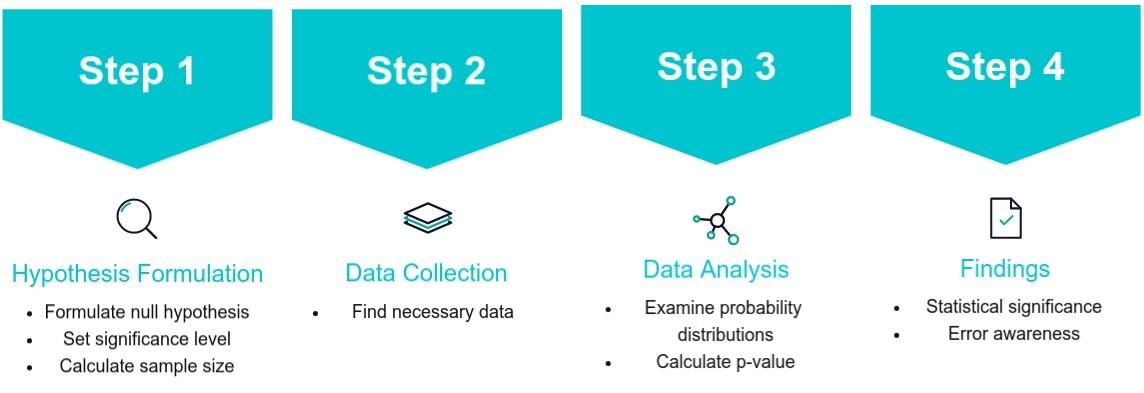
Hypothesis testing is the act of determining whether an hypothesis can be rejected (or not) based on real-life observations. The first step of this process (and consequently of A/B-testing) is to formulate the hypothesis you are going to be testing. For example, you might have an hypothesis that blog posts about statistics will bring less visitors than blog posts about programming. This would be called the alternative hypothesis.
However, in hypothesis testing the hypothesis being tested should be formulated in such a way that it indicates no relationship between the parameters being tested. Therefore the hypothesis should be formulated as blog posts about statistics will not bring less visitors than blog posts about programming. This type of hypothesis is called the null hypothesis. The reasoning behind formulating a null hypothesis is the same as the legal principle innocent until proven guilty – evidence is needed before making a claim. Just as you would need evidence to convict someone guilty of a crime, you need evidence to reject the null hypothesis. Depending on what hypothesis you are going to be testing, you can use different types of “evidence”.
In A/B-testing, the hypothesis should always include one independent variable with two different values (variants). In this example the independent variable is represented by blog topics and its values (variants) are statistics and programming.
The “evidence” that is used for testing the null hypothesis are two data sets, one for each variant. The variants are to be measured using a predefined metric called dependent variable. The term dependent indicates that this variable is affected by another (the independent) variable. In the example, the dependent variable is the number of visitors. All in all, our evidence will consist of two data sets containing the number of visitors for statistical blog posts vs the number of visitors for programming blog posts.
The fourth step of hypothesis testing is to set a significance level. We will discuss what this means in later sections. For now, we will just set the significance level to 0.05.
The last step before moving on to data collection is to do a power analysis. The aim of the power analysis is to determine an appropriate sample size that is not too small (meaning we might not detect differences between the variants) or too large (meaning we might detect insignificantly small differences between the variants). This is a step which I will not cover thoroughly in this blog, since it is a topic worthy of its own blog post.
For now it will be enough to know that the statistical power of the test must be decided before doing this analysis. Statistical power is the probability of finding an effect when there is one, i.e. rejecting the null hypothesis when it is incorrect, and is typically set to 0.8.
The outcome of the power analysis for the blog post example tells me that I need at least 900 visitors in each group to detect a difference that I find sufficient.
With these steps complete, we are soon ready to move on. First, let’s just take a brief recap of the steps we have taken thus far:
- Formulate a null hypothesis.
- Select two variants (A and B) for the independent variable.
- Select a dependent variable.
- Select a significance level.
- Calculate appropriate sample size.
Now that we have made sure that those five steps are complete, let’s move on!
Data Collection
The data collection phase includes setting up and conducting an experiment, where observation groups are divided based on the independent variable and evaluated using the dependent variable. In web analytics this is often done via softwares such as Google Optimize. As I don’t want to dig too deep into practicalities, I will not set up an actual experiment in this blog. Instead, I will move straight on to the expected output of the data collection phase – the two data sets needed to test the null hypothesis.
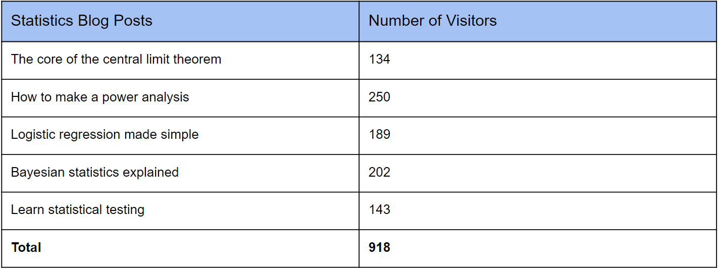
For illustration purposes, I have created two dummy data sets based on the earlier example of blog posts. The first data set contains information about five statistics blog posts and how many readers each post had:
The second data set contains information about five programming blogs and how many readers each post had:
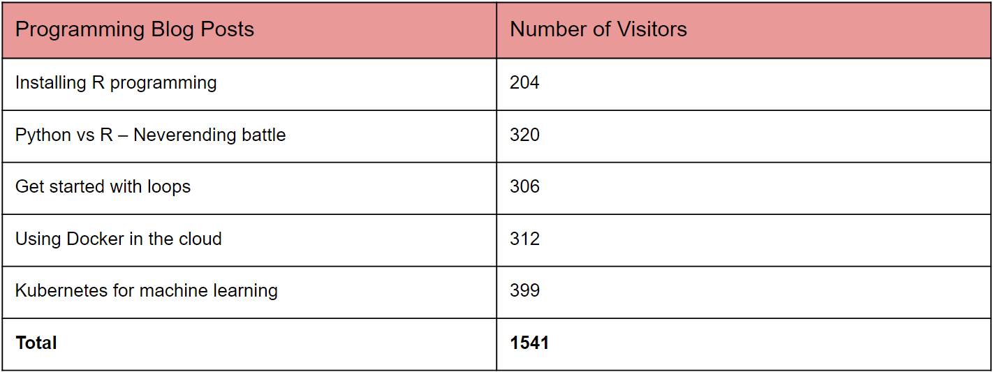
As can be seen from these data sets, there were a total of five samples (blog posts) of each variant. Although an equal split is not necessary, it is generally a good practice. Each observation was measured using the dependent variable (number of visitors). What we will do next is to analyse our data to see if there is any difference between the two groups.
Data Analysis
To compare the measurements from the two variants (and to determine whether the null hypothesis can be rejected), some calculations must be made on the collected data. But before making any calculations it is essential to understand what we will be calculating. Therefore we must first talk about probability distributions.
Probability Distributions
A probability distribution is a function of the probability of random outcomes occurring. The probability distribution is usually depicted in a graph with the probability of an outcome on the y-axis and the outcomes on the x-axis.
A simple example of a probability distribution is that of a coin flip. Flipping a coin has only two outcomes: heads or tails. The probability of heads when flipping a coin is 0.5 (50%) which is the same as that of tails. Since the probability of the two outcomes occurring are the same, the probability distribution shows two boxes of the same height (this could also be represented by a flat line instead of boxes).
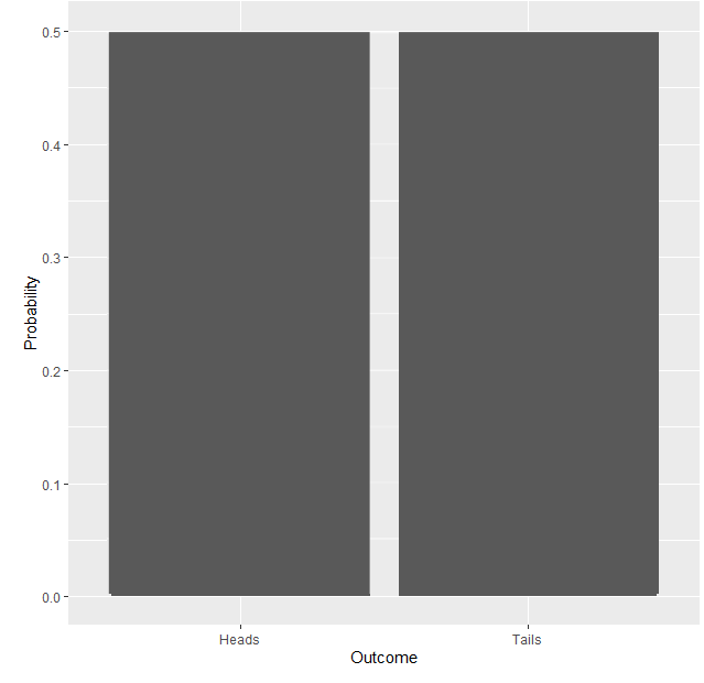
Although if you were to conduct a coin flip experiment yourself, it is unlikely that you would flip exactly the same number of heads and tails, thus the probability distribution of your experiment would be a (slight) misrepresentation of the true probability distribution. As we are about to see, the more observations (coin flips) that you collect in your experiment, the closer its probability distribution will resemble the true probability distribution.
Let’s look at a quick example to show this principle using R programming. I have created a script that outputs a box plot representing the probability distribution of a coin flip experiment.
The first simulation includes only 10 coin flips:

As we can see, this experiment is pretty far off the 50/50 split of the true distribution. Our experiment shows that the probability of heads is 0.7 while the probability of tails is only 0.3.
In the second experiment we increase the observations to 100 coin flips:

Here we are getting a lot closer to depicting the actual distribution of a coin flip, although the probability of heads is somewhat higher than that of tails (about 55/45 split).
Finally, let’s ramp up our experiment to a massive 100 000 coin flips:
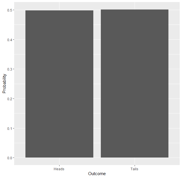
Now we can see that the split is almost even, only differing a fraction of a percent. These three experiments show that the probability distribution of an experiment converges toward the true probability distribution as the sample size is increased. Although this is far from surprising, it reminds us of the importance of selecting an appropriate sample size. Of course, there will be a trade-off between accuracy and time efficiency, but you want to make sure that you collect enough data to not be fooled by chance.
Even though a coin flip experiment is a good starting point, it is rather different than the types of experiments you are likely to be testing. So let’s once again have a look at our earlier example of blog post topics.
Unlike coin flips, the number of outcomes (readers of a blog) could be any number. Instead of using two bars to represent the possible outcomes we will use a line. As we can see from the collected data, the blog posts (both topics) seem to attract between 100-400 readers. With the data points we have collected, we can actually plot the probability distribution functions of the two topics:
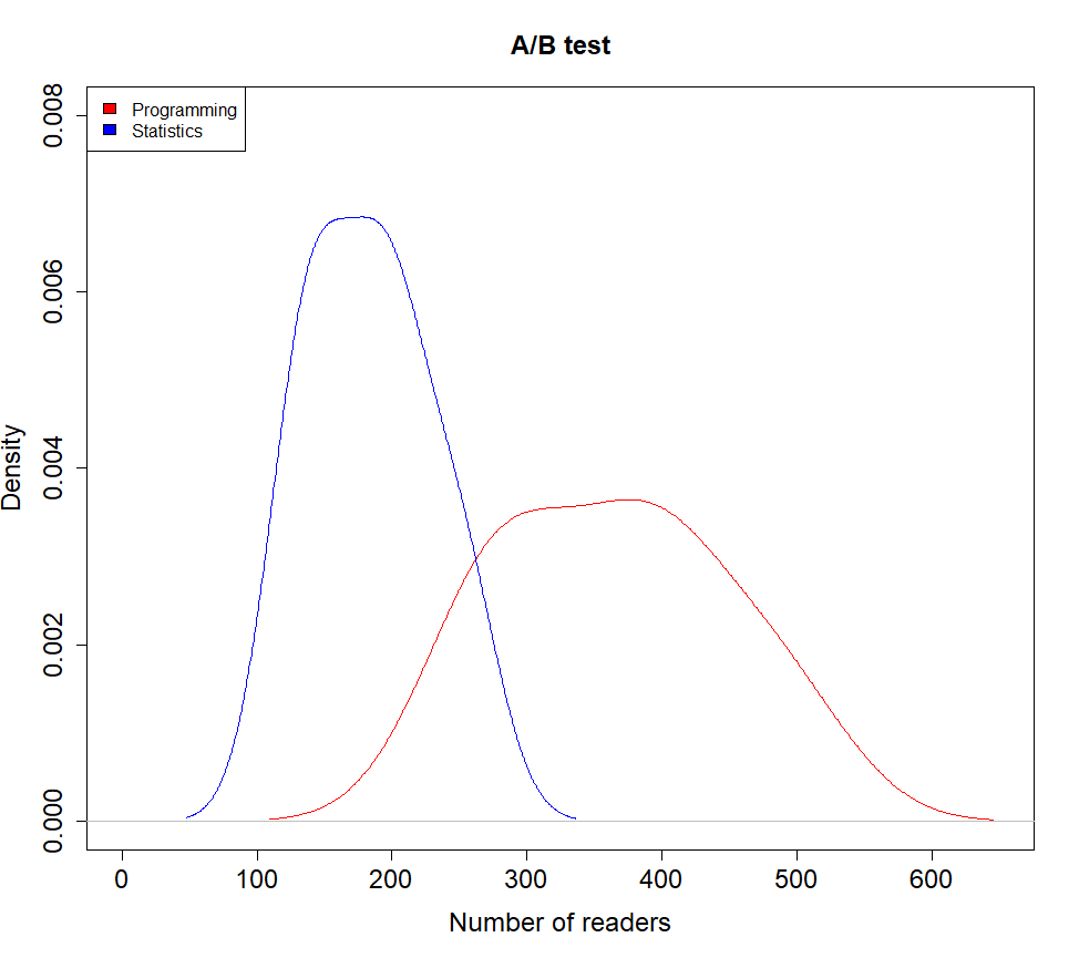
The x-values under the red line is representing the possible outcomes (number of readers) for programming blog posts while the x-values under the blue line represents the possible outcomes (number of readers) for statistics blog posts. The highest point on the red curve is the most likely number of readers that a programming blog post is to generate. This number is about 400 readers. The most likely number of readers for a statistics blog post is about 180 readers. The area under the curve (the integral) of each plot is equal to one, which is the same to say that the density curve includes all possible outcomes.
When conducting an A/B-test, you are actually trying to determine whether the samples of the A and B groups belong to the same probability distribution. From the two density curves above it is alluring to conclude that the samples from the A and B groups are from different distributions. This might be true. However, if we were to collect more samples the two curves might start to melt together. Remember the first coin flip experiment where only 10 coins were flipped. The probability distribution of that experiment differed very much from the true distribution, and it could be the same situation here.
We can actually calculate the probability that the samples from the two groups belong to the same probability distribution. This brings us to the next section – p-values.
P-value
One of the most common terms when it comes to A/B-testing is p-value. It is an abbreviation of probability value, and is a variable that ranges from 0-1. The probability value measures the probability that the null hypothesis is true, which means that the samples from the A and B groups belong to the same probability distribution. A low p-value indicates a low chance that the null hypothesis is true, while a high p-value indicates the opposite.
If the samples of the groups do not belong to the same probability distribution, it means that the independent variable has a measurable effect on the dependent variable. It is very important to note that the p-value gives no indication of how strong an effect the independent variable has upon the dependent variable. Thus, the independent variable could have an extremely little effect on the dependent variable even if the p-value is extremely low. This is crucial to remember, and is something that is often misunderstood.
How to calculate the p-value depends on what the probability distribution looks like. For example, you would calculate the p-value of a binomial distribution differently to that of a normal distribution. The probability distributions in the blog post example closely resembles a normal (Gaussian) distribution. In this case we can use a t-test to calculate the p-value. If you would do this by hand, you would first calculate the t score, and then look up the p-value in a table. Nowadays you don’t need to calculate the p-value by hand, instead this is often done automatically in A/B testing tools, such as Google Optimize.
Using Welch’s t test in R, the p-value for the blog example is calculated to 0.006. This means that the probability of the null hypothesis being true (and also the two groups belonging to the same distribution) is about 0.6%. Therefore it is highly unlikely that statistics blog posts draw as many readers as programming blog posts.
Findings
So we are getting close to completing our A/B-test. All the calculations have been made, and now we only need to take a last look at our data to see what our findings were.
Remember that we set a significance level in the first section of the post, just after deciding our null hypothesis? Now it is time to explain why this was done, and how it will help us interpret our findings.
Statistical Significance
The significance level is a threshold that the p-value must be equal to or less than in order to reject the null hypothesis. It is often denoted as the greek letter alpha (α), and is typically set to 0.05 or lower. If the p-value is equal to or less than the significance level, the test results are significant. Note that statistical significance is not a universal metric, but depends entirely on the chosen significance level. If an abnormally high significance level is set (for example 0.5), test results would be statistically significant as long as the p-value is below 0.5 even though this would only mean a 50% chance that the null hypothesis would be false. Hence, it is a good practice to look at the actual significance level of an experiment rather than blindly trusting “statistically significant” results.
Sometimes you will get into situations where the p-value is just above the significance level. Then it will be very tempting to increase the significance level a bit to get “significant” results. This would completely invalidate your test results, which is why you must always resist the urge to change the significance level retroactively.
Since the p-value in the blog post example was well below the significance level of 0.05, the test results are significant. We can actually say that statistics blog posts draw less readers than programming blog posts. Remember that even though the test results are significant, it is still a (small) chance that the results could be wrong. This is why we need to be mindful of test errors.
Error Awareness
In hypothesis testing, there are two types of errors related to incorrect conclusions about the null hypothesis – Type I and Type II errors.
Type I error is when the null hypothesis is falsely rejected, i.e. it is concluded that the independent variable has an effect on the dependent variable even though it has not. In the example, this would correspond to concluding that statistics blog posts draw less readers than programming blog posts, even though there is no such correlation.
Type II error is the opposite scenario where the null hypothesis is not rejected even though the independent variable has an effect on the dependent variable. In the example, this would correspond to concluding that statistics blog posts are not drawing less readers than programming blog posts, even though they actually are. Increasing the statistical power of the test will decrease the risk of type II errors.
What is tricky about errors is that you probably won’t know if they occur. This is why science seldom lay trust in single studies, but instead examines relationships over multiple studies. For A/B testing, you are unlikely to be conducting the same experiment multiple times, which is why you have to live with the chance that the test results could be faulty.
If implementing the winning variation of an A/B test could have a huge impact on your business, you probably want to decrease the significance level or conduct multiple tests to minimize the risk of making an incorrect decision.
With the potential errors of hypothesis testing covered, the A/B test is now completed. Before ending this blog post, I would like to write down a few summarizing thoughts around A/B testing.
Summary
As you can see there are many components of A/B testing to get acquainted with. It may not be necessary to know each and every one of these in full detail, but I am sure that they will help you create better and more accurate tests if understood.
With third party tools making the process of setting up tests ever easier, the knowledge of what is being done behind the scenes is decreasing. I have seen many A/B tests being conducted in ways that fully invalidates the results. This is dangerous as it leads people and companies to make decisions based on chance (at best) rather than data driven insights.
‘Data driven’ has become such a misused term since the data behind the decisions is all too often misinterpreted. By investing a couple of hours in statistics and getting an even better understanding of fundamental statistical principales, you can make sure that your decisions are based on science and truly use A/B testing as a means for constant improvement.
Thank you for reading, and please leave a comment if there is anything you would like to discuss!

